TOC
Introduction
This is a sample data blog, where in I will be working with one of the most famous & processed dataset in Data analytics & ML community mtcars. The comments & workings would be around the dataset, hence it is advisable to go through the dataset once.
mtcars dataset –> 32 rows & 11 columns, column names as below:
[, 1]   mpg     Miles/(US) gallon
[, 2]   cyl     Number of cylinders
[, 3]   disp    Displacement (cu.in.)
[, 4]   hp      Gross horsepower
[, 5]   drat    Rear axle ratio
[, 6]   wt      Weight (lb/1000)
[, 7]   qsec    1/4 mile time
[, 8]   vs      Engine (0 = V-shaped, 1 = straight)
[, 9]   am      Transmission (0 = automatic, 1 = manual)
[,10]   gear    Number of forward gears
[,11]   carb    Number of carburetors
mtcars dataset
Download data set here
Read about the variables here
Break the Syntax
This is an important section, if you want to just skim through what I have done & not getting details of things.
Anything written in red is the question which I will answer during the post
#Anything written under this grey box is R Code & its output Anything written like this is the comment on output produced
Anything written like this is hyperlinked for further readings
Anything written like this is to just get your attention
Anything left are the Images or output produced (I am sure you can identify them :) For example refer plot 1
Figure 1: A fancy pie chart.
Lets get started
Data Exploration
The initial bit where we are getting familiar with dataset is called Data Exploration phase. In this stage, we check the dimensions (rows,columns) of the dataset, view first few rows to get an idea of how data is structured, check summary alongside plethora of other steps. Let’s do some exploration on mtcars dataset.
- Checking the dimensions then Viewing the first 10 rows of the data
library(tidyverse)
library(broom)
library(knitr)
library(printr)

dim(mtcars)
[1] 32 11kable(head(mtcars),align = 'c')| mpg | cyl | disp | hp | drat | wt | qsec | vs | am | gear | carb | |
|---|---|---|---|---|---|---|---|---|---|---|---|
| Mazda RX4 | 21.0 | 6 | 160 | 110 | 3.90 | 2.620 | 16.46 | 0 | 1 | 4 | 4 |
| Mazda RX4 Wag | 21.0 | 6 | 160 | 110 | 3.90 | 2.875 | 17.02 | 0 | 1 | 4 | 4 |
| Datsun 710 | 22.8 | 4 | 108 | 93 | 3.85 | 2.320 | 18.61 | 1 | 1 | 4 | 1 |
| Hornet 4 Drive | 21.4 | 6 | 258 | 110 | 3.08 | 3.215 | 19.44 | 1 | 0 | 3 | 1 |
| Hornet Sportabout | 18.7 | 8 | 360 | 175 | 3.15 | 3.440 | 17.02 | 0 | 0 | 3 | 2 |
| Valiant | 18.1 | 6 | 225 | 105 | 2.76 | 3.460 | 20.22 | 1 | 0 | 3 | 1 |
We observe that the dataset contains 32 rows & 11 columns. The column names are shortened due to lengthy names but a fair idea can be derived from that they could mean. (To read more about description of variable click link mentioned above)
For ex:-
mpg –> Miles/(US) gallon
disp –> Displacement (cu.in.)
- Summary & structure of the dataset
str(mtcars)'data.frame': 32 obs. of 11 variables:
$ mpg : num 21 21 22.8 21.4 18.7 18.1 14.3 24.4 22.8 19.2 ...
$ cyl : num 6 6 4 6 8 6 8 4 4 6 ...
$ disp: num 160 160 108 258 360 ...
$ hp : num 110 110 93 110 175 105 245 62 95 123 ...
$ drat: num 3.9 3.9 3.85 3.08 3.15 2.76 3.21 3.69 3.92 3.92 ...
$ wt : num 2.62 2.88 2.32 3.21 3.44 ...
$ qsec: num 16.5 17 18.6 19.4 17 ...
$ vs : num 0 0 1 1 0 1 0 1 1 1 ...
$ am : num 1 1 1 0 0 0 0 0 0 0 ...
$ gear: num 4 4 4 3 3 3 3 4 4 4 ...
$ carb: num 4 4 1 1 2 1 4 2 2 4 ...summary(mtcars)| mpg | cyl | disp | hp | drat | wt | qsec | vs | am | gear | carb | |
|---|---|---|---|---|---|---|---|---|---|---|---|
| Min. :10.4000 | Min. :4.0000 | Min. : 71.100 | Min. : 52.000 | Min. :2.76000 | Min. :1.51300 | Min. :14.5000 | Min. :0.0000 | Min. :0.00000 | Min. :3.0000 | Min. :1.0000 | |
| 1st Qu.:15.4250 | 1st Qu.:4.0000 | 1st Qu.:120.825 | 1st Qu.: 96.500 | 1st Qu.:3.08000 | 1st Qu.:2.58125 | 1st Qu.:16.8925 | 1st Qu.:0.0000 | 1st Qu.:0.00000 | 1st Qu.:3.0000 | 1st Qu.:2.0000 | |
| Median :19.2000 | Median :6.0000 | Median :196.300 | Median :123.000 | Median :3.69500 | Median :3.32500 | Median :17.7100 | Median :0.0000 | Median :0.00000 | Median :4.0000 | Median :2.0000 | |
| Mean :20.0906 | Mean :6.1875 | Mean :230.722 | Mean :146.688 | Mean :3.59656 | Mean :3.21725 | Mean :17.8487 | Mean :0.4375 | Mean :0.40625 | Mean :3.6875 | Mean :2.8125 | |
| 3rd Qu.:22.8000 | 3rd Qu.:8.0000 | 3rd Qu.:326.000 | 3rd Qu.:180.000 | 3rd Qu.:3.92000 | 3rd Qu.:3.61000 | 3rd Qu.:18.9000 | 3rd Qu.:1.0000 | 3rd Qu.:1.00000 | 3rd Qu.:4.0000 | 3rd Qu.:4.0000 | |
| Max. :33.9000 | Max. :8.0000 | Max. :472.000 | Max. :335.000 | Max. :4.93000 | Max. :5.42400 | Max. :22.9000 | Max. :1.0000 | Max. :1.00000 | Max. :5.0000 | Max. :8.0000 |
Here we explore two other things related to dataset
The structure of the mtcars data, which we can are all numeric column. To read up more on data structures, check this link
The summary of the dataset, since all columns are numeric we get to see an overview of broad stastical parameters like mean, median, mode etc.
Data Visualization
Let’s say we want to analyse what is the relationship between mpg(miles per gallon) & hp (horse power) in different cyl (cylinder types)
mtcars %>%
  ggplot(aes(x=mpg, y=hp, color=as.factor(cyl)))+
  geom_point()+
  labs(title="Relationship between mpg & hp",
       subtitle = "We can observe that as number of cylinders increases so does mpg but horse power decreases",
       x="Miles Per Gallon",
       y="Gross Horse Power ",
       color="Number of cylinders")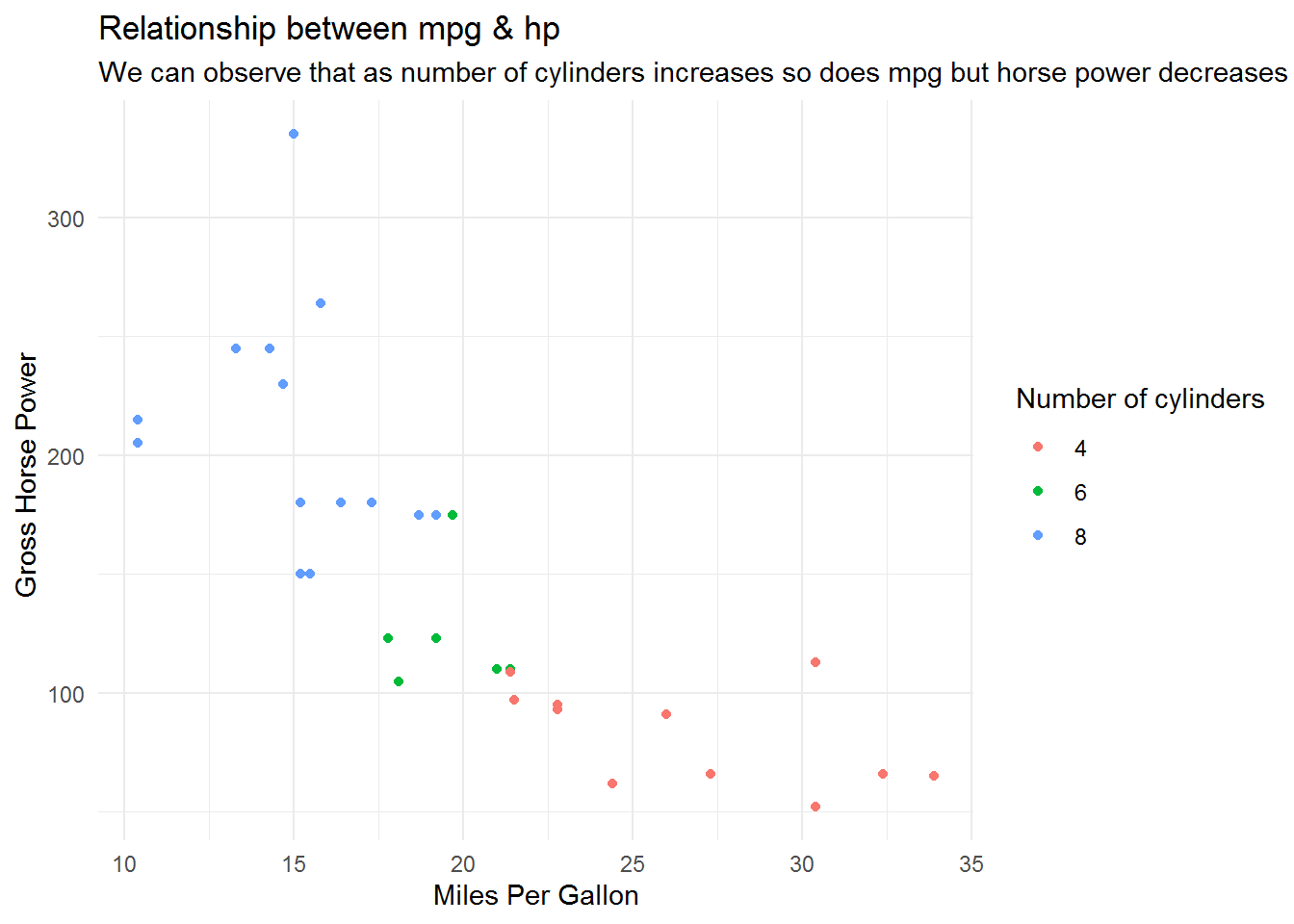
Linear Regression
This would be the last section for this intro post. Lets quickly see that if we have to predict mpg using all other variables which variable would be most important feature in our prediction. While there are many alogrithms to do this, we would be using linear regression in this post.
head(mtcars)| mpg | cyl | disp | hp | drat | wt | qsec | vs | am | gear | carb | |
|---|---|---|---|---|---|---|---|---|---|---|---|
| Mazda RX4 | 21.0 | 6 | 160 | 110 | 3.90 | 2.620 | 16.46 | 0 | 1 | 4 | 4 |
| Mazda RX4 Wag | 21.0 | 6 | 160 | 110 | 3.90 | 2.875 | 17.02 | 0 | 1 | 4 | 4 |
| Datsun 710 | 22.8 | 4 | 108 | 93 | 3.85 | 2.320 | 18.61 | 1 | 1 | 4 | 1 |
| Hornet 4 Drive | 21.4 | 6 | 258 | 110 | 3.08 | 3.215 | 19.44 | 1 | 0 | 3 | 1 |
| Hornet Sportabout | 18.7 | 8 | 360 | 175 | 3.15 | 3.440 | 17.02 | 0 | 0 | 3 | 2 |
| Valiant | 18.1 | 6 | 225 | 105 | 2.76 | 3.460 | 20.22 | 1 | 0 | 3 | 1 |
linear <- lm(mpg~. , data=mtcars)

tidy(summary(linear))| term | estimate | std.error | statistic | p.value |
|---|---|---|---|---|
| (Intercept) | 12.303374156 | 18.717884429 | 0.657305808 | 0.518124397 |
| cyl | -0.111440478 | 1.045023363 | -0.106639222 | 0.916087376 |
| disp | 0.013335240 | 0.017857500 | 0.746758487 | 0.463488650 |
| hp | -0.021482119 | 0.021768579 | -0.986840654 | 0.334955314 |
| drat | 0.787110972 | 1.635373069 | 0.481303616 | 0.635277898 |
| wt | -3.715303928 | 1.894414300 | -1.961188706 | 0.063252151 |
| qsec | 0.821040750 | 0.730844796 | 1.123413280 | 0.273941270 |
| vs | 0.317762814 | 2.104508606 | 0.150991454 | 0.881423472 |
| am | 2.520226887 | 2.056650553 | 1.225403549 | 0.233989711 |
| gear | 0.655413017 | 1.493259961 | 0.438914211 | 0.665206434 |
| carb | -0.199419255 | 0.828752498 | -0.240625827 | 0.812178713 |
Above, we can see that wt is the most important predictor as its p-value is the lowest. (Well, its not so simple, but we'll call off at this point this as of now)
That’s all Folks for the intro post. This was just an intro post to get first timers familiar with the syntax & flow of the data blogs. Incase, you would love to explore more detailed & advanced posts, head over to other post from home page
comments powered by Disqus